
Modo generated P50 solar generation profile
In the absence of a custom solar profile, we use the PVLib Python library to produce bespoke solar generation forecasts. The method integrates detailed equipment specifications, optimised system sizing, realistic weather data, and loss modelling to give representative, site-specific results.
Here's how it works:
1. Initial Configuration and Site Data
Solar forecasts begin with detailed, location-specific inputs:
- Geographic Coordinates: Latitude and longitude, essential for determining local irradiance patterns and weather conditions.
- System Configuration: Surface tilt and azimuth angles tailored to the project's physical installation.
2. Equipment Selection & Site Optimisation
We source detailed module and inverter specifications from the California Energy Commission (CEC) database. Angle-of-incidence (AOI) parameters, absent from the CEC database, are derived from the Sandia National Laboratories database.
We assume the following equipment in our modeling:
- Solar Modules: Trina Solar TSM-720NEG21C.20
- Inverters: Sungrow Power Supply SG2500U (550V)
These are then used to build up a realistic solar site which respects the user inputted data (AC and DC limits). The optimal solar array and site configuration is based on:
- Modules per String: Determined by inverter voltage limitations.
- Strings per Inverter: Based on inverter current capacity.
- Number of Inverters: Calculated to meet the target maximum power output.
This ensures the forecast accurately reflects realistic operational limits of installed systems.
4. Weather Data Integration
To generate realistic irradiance data, we leverage PVLib’s robust irradiation forecasting capabilities. The model uses the site’s latitude and longitude to access irradiance data from s PVGIS data, constructing a Typical Meteorological Year (TMY) that represents average historical weather conditions.
This approach mirrors the logic employed by PVsyst, the industry-standard solar modelling software.
5. Accounting for Losses
We model several loss factors that affect real-world solar performance:
-
Temperature Effects: Modelled via the Sandia photovoltaic array performance model (SAPM).
-
Loss Factors:
- Soiling
- Shading
- Mismatch
- Wiring losses
- Connection losses (scaled by system size)
- Availability-related downtime
These cumulative losses provide a realistic adjustment to theoretical maximum energy generation.
6. PV System and Model Chain Execution
Once we have set up the site and integrated equipment parameters, acquired weather data, and accounted for losses, we leverage the PVLib ModelChain framework to model final AC generation.
The model performs advanced calculations such as:
- Physical Angle-of-Incidence (AOI) adjustments
- Spectral irradiance variations
- Temperature-dependent performance shifts
- Loss modeling
Results
This detailed process results in a bespoke and realistic solar generation profiles for your site .
Our approach captures the significant differences in average irradiation throughput the country, with significant variations in solar generation between geographies.
Here's an example of generation profiles of two sites differing only by location (Inverness and Somerset). Unsurprisingly, Somerset sees more consistent, sunny conditions.
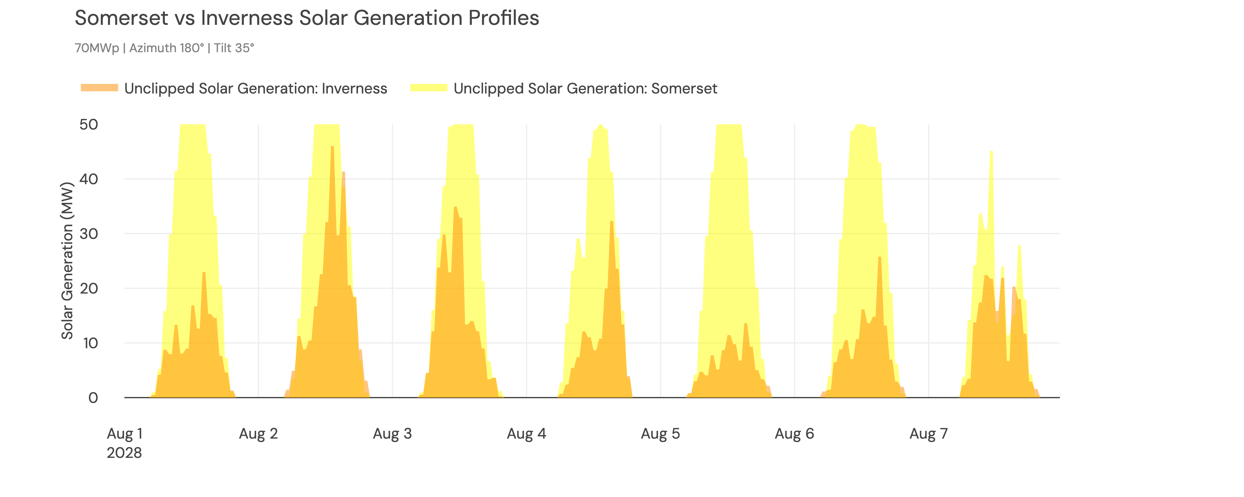
Example week of solar generation forecasts for identical sites in Inverness and Somerset
Whilst this is not the case throughout the entire year (some days see higher solar generation in Inverness), the annual load factor of the Somerset site is 17% higher than for Inverness.
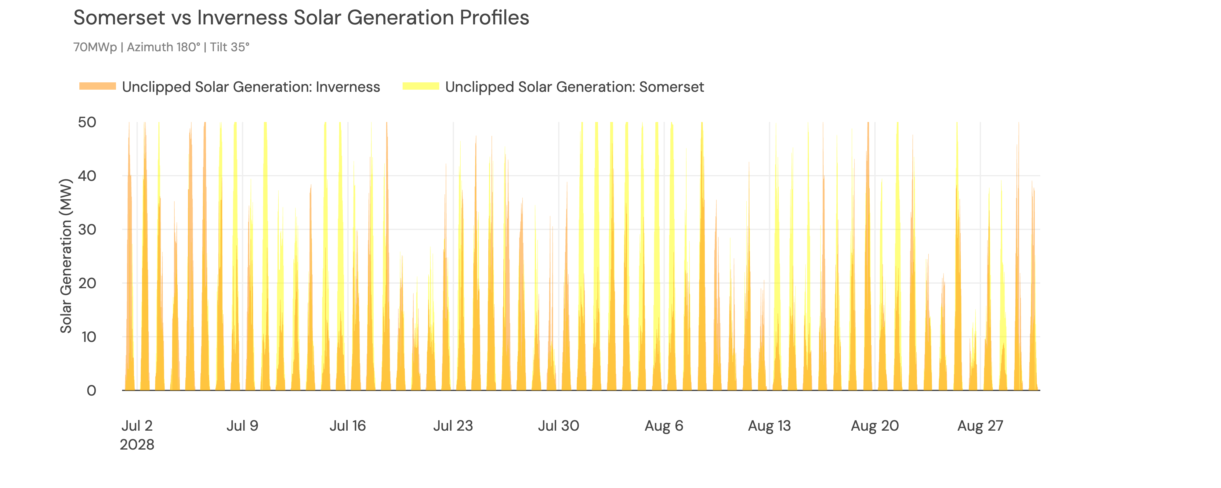
Example month of solar generation forecasts for identical sites in Inverness and Somerset
Updated 8 months ago
What’s Next
Once we've a created solar generation profile, it is shuffled to properly capture cannibalisation