New-build, Retrofit, and Retirement Decisions

We attempt to build a realistic evolution of the capacity stack given both net-zero goals but also current commercial (and operational) realities. For example, we do not forecast a system with no gas on it in 2035 as we see that would lead to loss of load - which we see as a red line.

Economics inform capacity growth and decline

Hurdle rates for NPV and IRR calculations are based on analysis by Europe Economics, with adjustments made to account for higher interest rates since this was published.

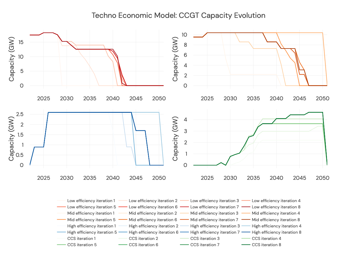
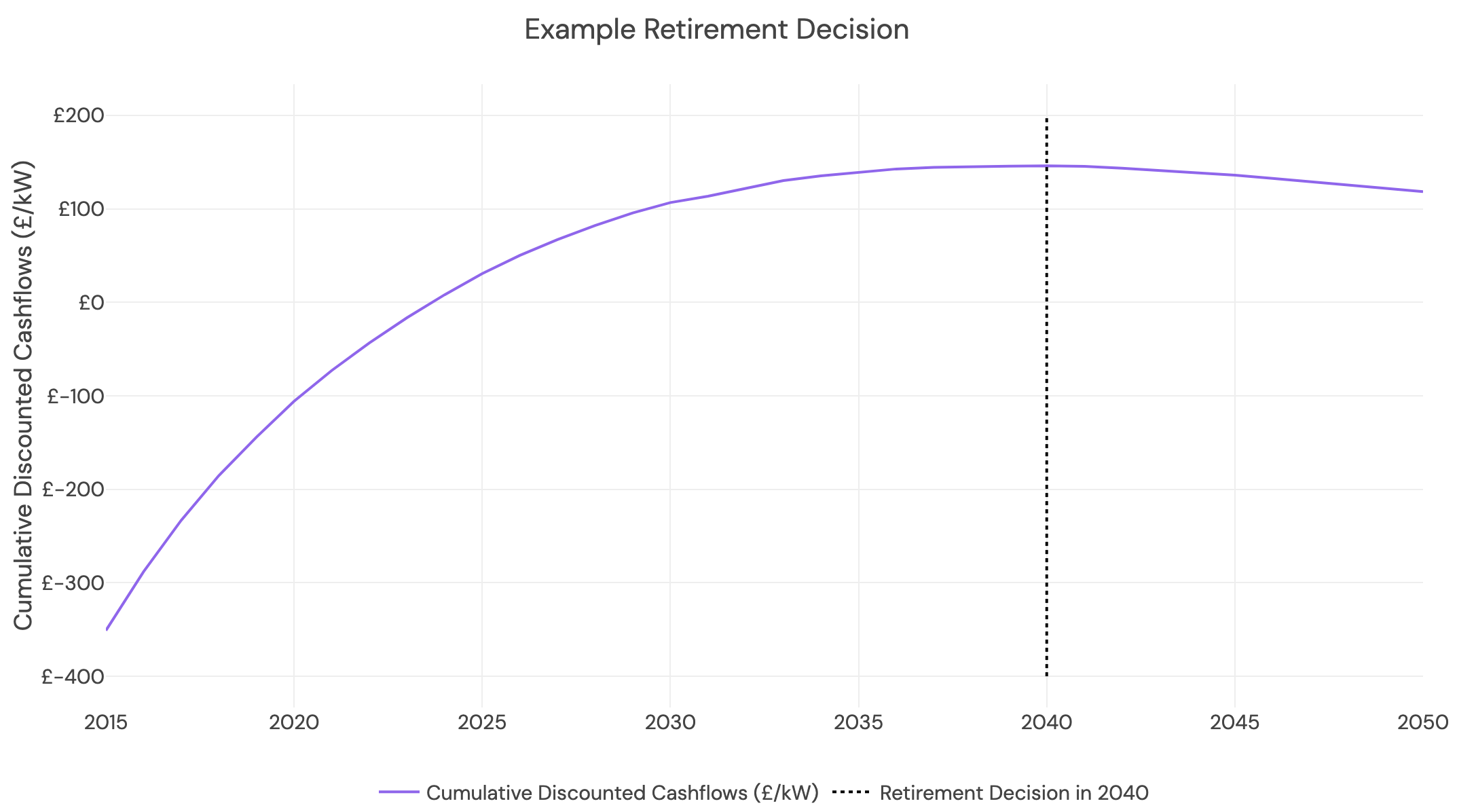
• We make retirement and retrofit decisions for unabated CCGTs. CCGTs that are not retrofitted with CCS are retired in the year of their maximum cumulative cashflows. A plant is retrofitted with CCS if it is technically feasible:
  • close to a planned carbon storage cluster,
  • profitable (NPV is greater than 0),
  • preferable to continued unabated generation (i.e., there is a higher NPV for retrofit).
• We make new build decisions for abated CCGTs (ie CCS). New abated CCGT plants are built when IRR exceeds the hurdle rate. We allow a maximum of 3 abated CCGT build decisions in each model iteration (ie across the forecast horizon). We assume that newly built unabated CCGT plants have a capacity of 0.9 GW. For the first 5GW of CCS, we assume a hurdle rate of 0%. For every subsequent GW that is built, we assume an incremental jump in the hurdle rate of 0.3% as the technology matures.
• We make new-build decisions for gas reciprocating engines. New plants are built when IRR exceeds the hurdle rate. New-build gas reciprocating engines have capacities of 100MW, and we allow a maximum of 10 new-build decisions for each, in each iteration. Existing OCGTs and gas reciprocating engines are retired in the year of their maximum cumulative cashflows. We don't build any new OCGTs.
• We make new build decisions for batteries. New batteries are built when IRR exceeds the hurdle rate. We allow a maximum of 10 new-build decisions over the time horizon per iteration, and apply a learning rate to the capacity of batteries we can build per year, starting at 3GW and by 2040 this is 4.8GW. We assume that newly built batteries have a capacity of 0.2 GW.

For example, when we say we allow 10 new build decisions for storage in each model iteration, it means we could build 10 new batteries in iteration 1, i.e., 1 per year from 2030 to 2040. In iteration 2, we build another 10 - giving 2 per year from 2030 - 2040. This could push spreads down in the price model - reducing IRR - so in iteration 3 we get 1 per year from 2030 - 2037, ie 7 new systems. Or, 17 new systems in total.

As we loop through multiple iterations of the model, it converges on a suitable build-out: one that responds to system needs without saturating the revenues (causing low IRRs) and avoids an overbuild.

All decisions are reversible. This means that any under or overbuild of a generation type can be corrected in the next iteration. This results in an iterative process where capacity build-out converges to an optimal solution.