
GB price, modelled without storage or interconnection
First of all, for each half hour, we create a supply curve and overlay demand. The marginal unit sets the price.
In a single half-hour period, we create a supply stack of available generation capacity, and rank it by short-run marginal cost.
We overlay demand.
The price is set where the two meet.
Where supply meets demand, the last unit to get us there sets the price - ie, the marginal unit.
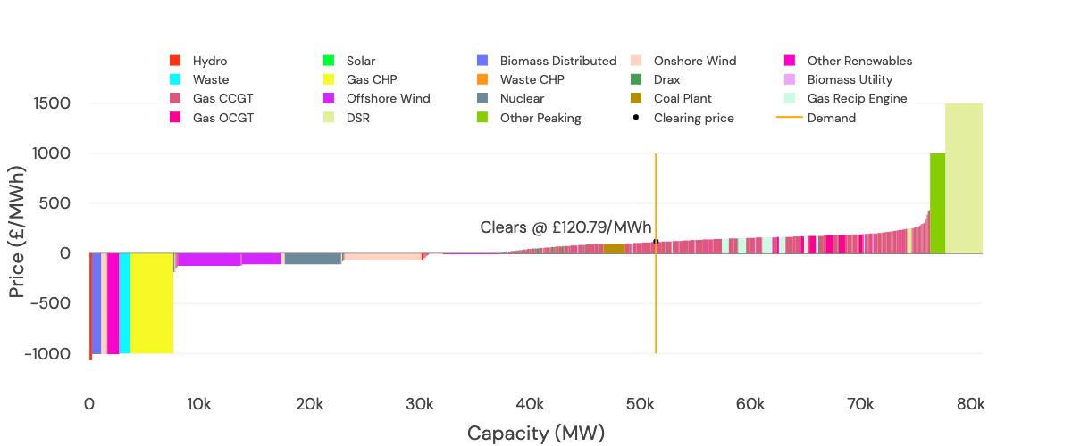
Example GB only Supply stack without storage or interconnectors. Source: Modo Energy
Our input data is not down to plant level, so we create a spline (or a linear fit) between the different technology sub-types to mimic plant-level price differences. It also means our resulting price curve is reasonably smooth when we do this across all half-hours.
Result: when there is a lack of capacity, we get high prices
Typically when wind and solar are low, and demand is high, we get very high prices. Remember, this is without storage or interconnectors. Those are added in next.

With no storage or interconnection, there are a lot of very high prices!
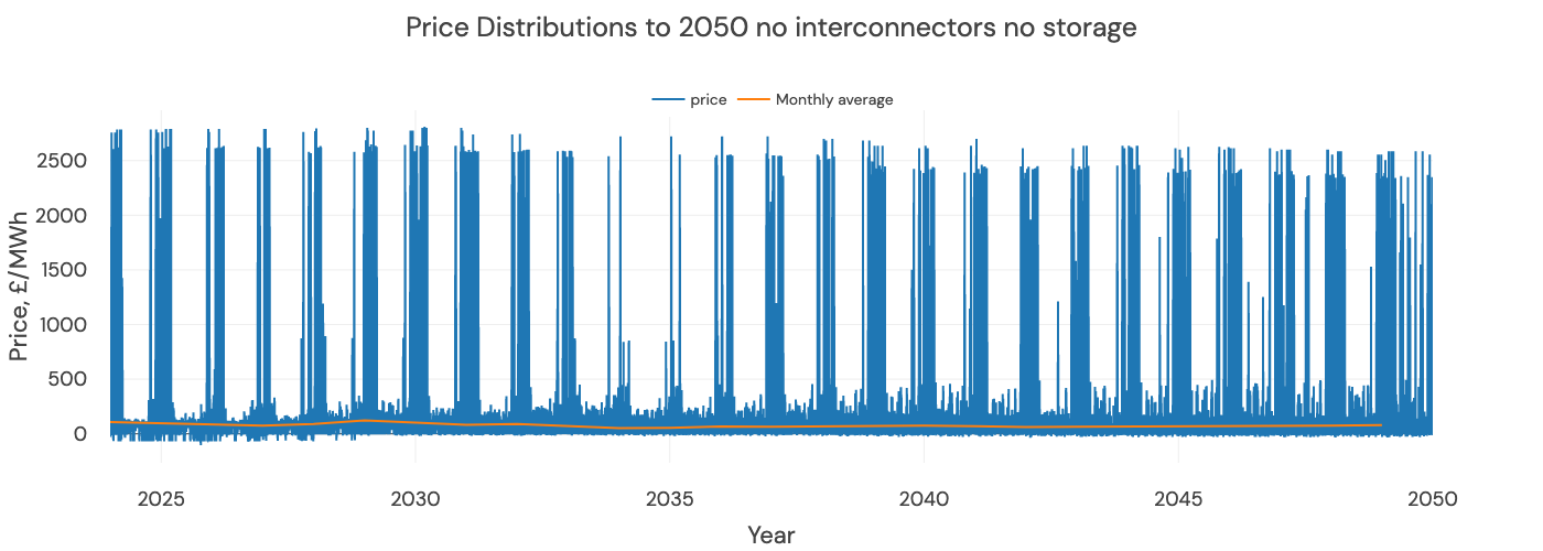
While interesting, clearly this does not model reality. Storage and interconnection ease capacity constraints on the system.
Updated 8 months ago
What’s Next
Check out how we add storage from batteries, pumped hydro and other technologies to the supply stack