Capturing cannibalisation

It's vital that the solar generation profile used to calculate revenues properly reflects the weather assumptions used to generate the underlying power prices. Otherwise, cannibalisation will not be properly captured and solar revenues will be systematically overestimated.

Aligning Solar Forecasts with our Fundamentals Model

The Problem

Our fundamentals model (FM) produces the power prices used in the solar revenue forecasts. Because the FM’s inputs are based on 2018 as the weather year, its power price outputs are inherently linked to the irradiance (sunniness and cloudiness) patterns of 2018.

In the solar revenue model, however, we either use a custom solar profile or one generated in PVLib. These profiles are not constrained to the 2018 weather year. If we overlay such a profile on top of the FM’s power prices, the two become misaligned. Without steps to address this mismatch, we risk attributing high solar output to days when the FM assumes low solar output and higher power prices. This would lead to an underestimation of cannibalisation effects and an overestimation of capture prices.

The comparison below illustrates the issue: the reference 2018 solar data used in the FM and the TMY profile generated in PVLib do not align

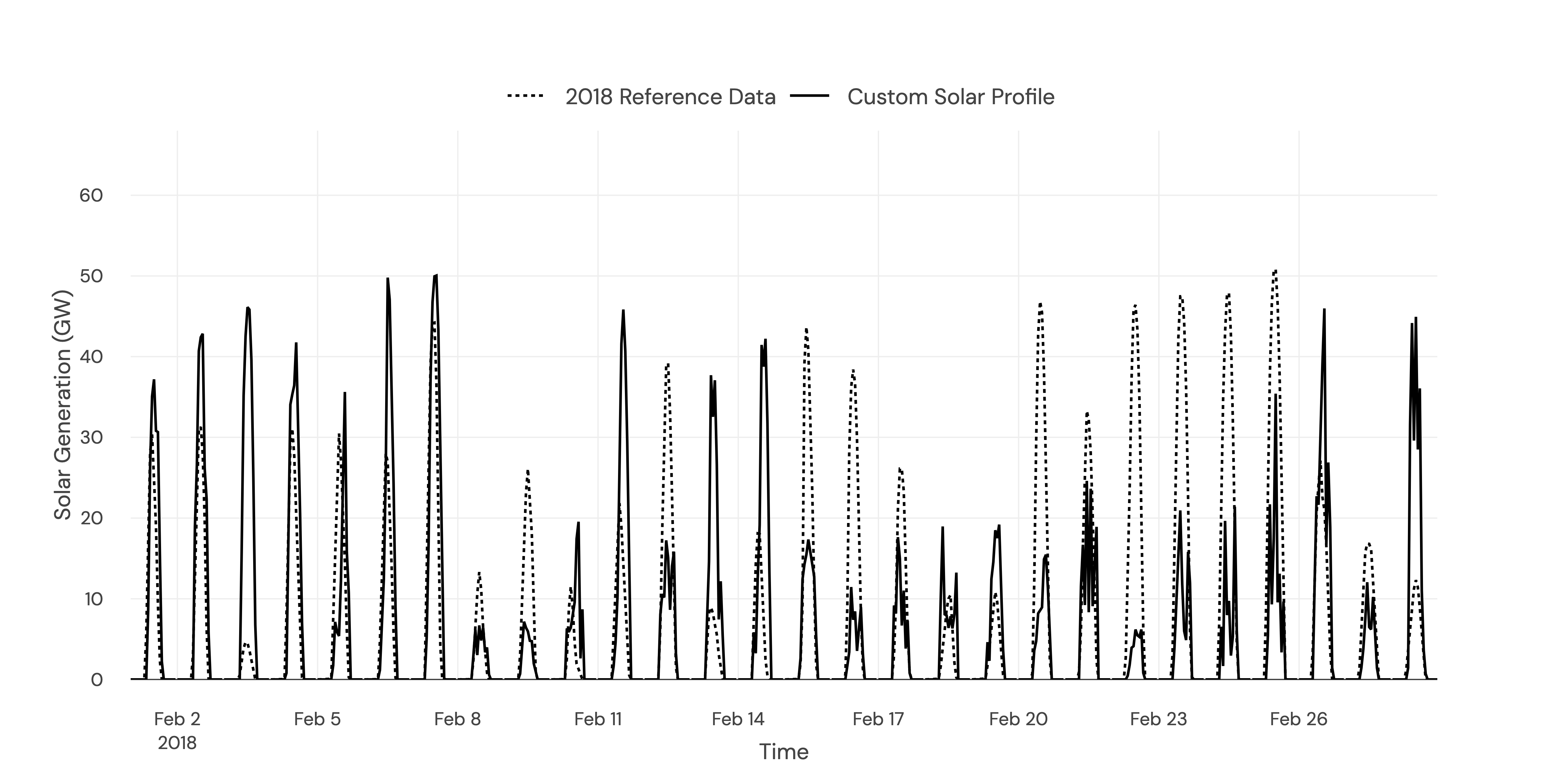
Example comparison between a custom solar generation profile (generated with PVlib) and 2018 reference data (generated by renewables ninja)

The Solution

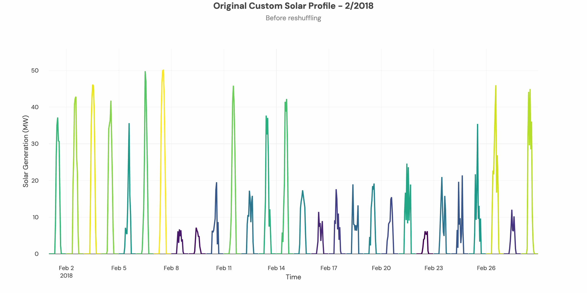
To address this, we shuffle the custom solar profile within each month to ensure it better aligns with the 2018 weather year used in the Fundamentals Model.

For each month, we:
• Generate a reference solar profile for 2018 at the site.
• Rank the days in the 2018 profile by total solar generation.
• Rank the days in the input solar profile (whether custom or PVLib-generated) by total solar generation.
• Reorder the days in the input profile to match the 2018 ranking.

This process ensures that solar output and power prices are consistently based on the same underlying weather patterns.

The example below illustrates the method applied to a PVLib-generated solar forecast:

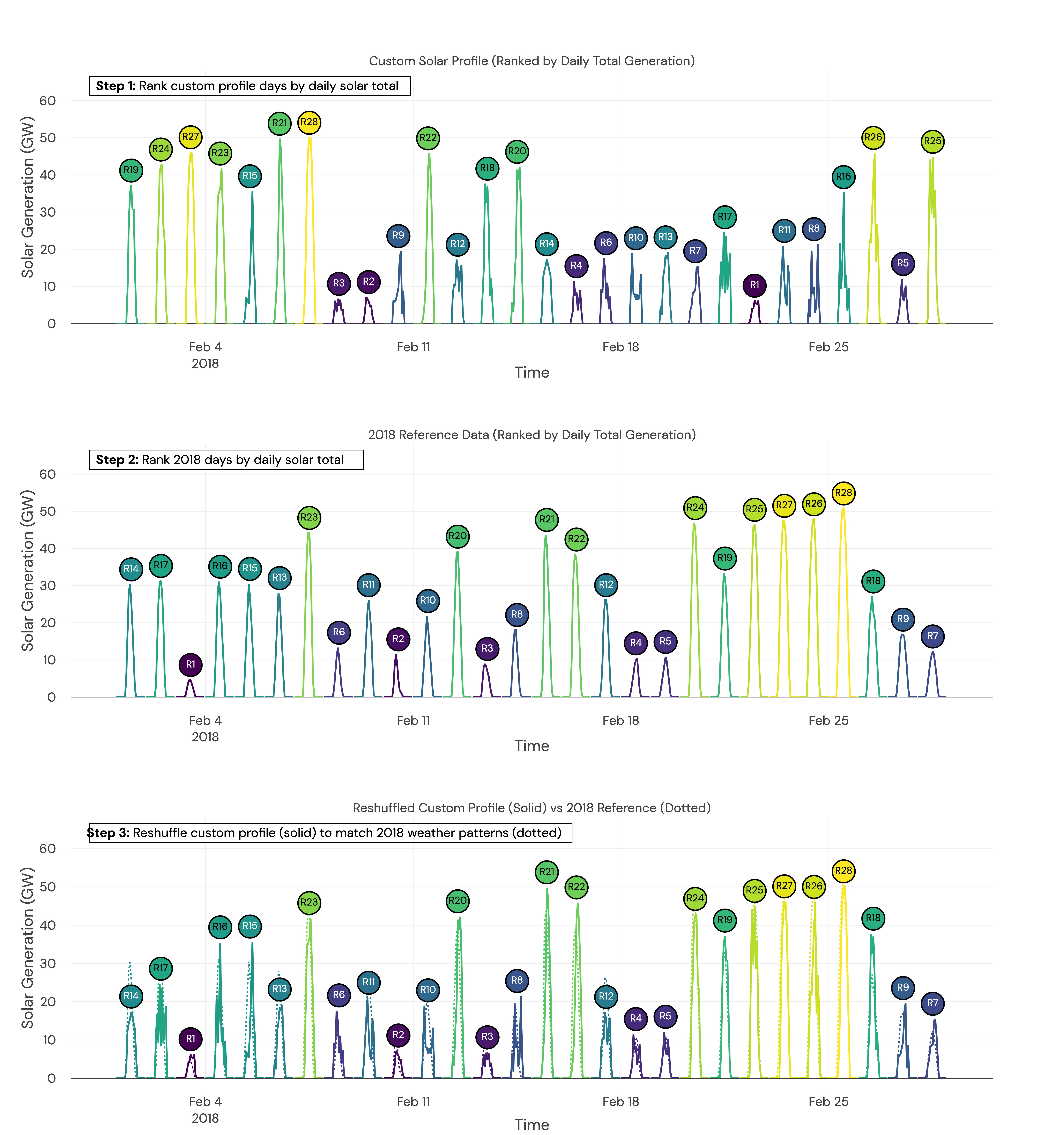
Example of custom solar profile shuffling logic. Shows a) Example custom solar profile where days of have been ranked by total solar generation b) 2018 reference data from renewables ninja (which matches the weather inputs in the fundamental model) where days of have been ranked by total solar generation c) Custom solar profile shuffled to match the ranking of the 2018 reference data

And here's the logic in action on the same example data:

Shuffling an example solar profile to align with 2018 reference data

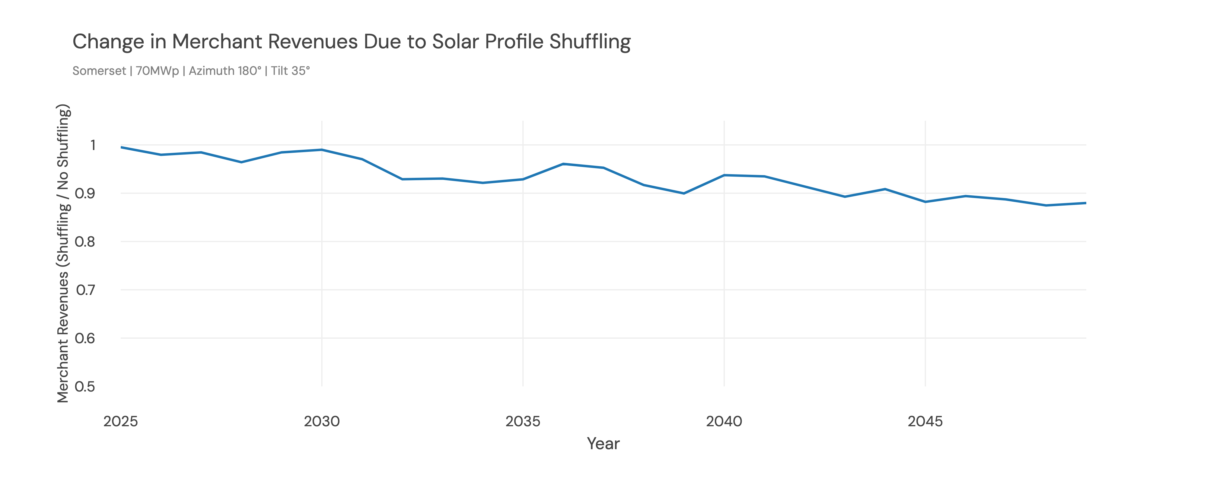
Why does this matter?

The shuffling logic has a material impact on merchant revenues and capture rates.

In this example, by 2045, merchant revenues are over 10% lower when the shuffling logic is applied.

If cannibalisation is not modelled correctly, solar revenues can be significantly overestimated.